In order to merge results from different surveys, for example customer satisfaction surveys for an entire year, you need to do some manual work in Excel, Google Sheets or any other spreadsheet editor such as LibreOffice Calc. The first half of this article is a step-by-step guide on how to create a macro in MS Excel and how to use it to merge results. The second half of the article teaches you how to create a pivot table in Google Sheets to view results from different surveys.
TABLE OF CONTENTS
Excel - Visual Basic macro
Start by downloading the individual results of each survey you want to merge. Store them in an easy to remember location on your PC.
Next, open Excel, and create a new document that acts as your main/master file. If you want to visualise a summary from all individual reports, rename the first tab Summary data, or something similar to differentiate it from the individual data sets.
The master file must be saved as a .xlsm (macro-enabled workbook).
Ensure that your source files (the excel reports you just downloaded) are not already open in Excel.
How to create a macro
Open the Visual Basic Editor. The default shortcut is Alt + F11
Right-click ThisWorkbook on the left then click Insert → Module


Paste this code in the window that appears, and Click CTRL+S to save.
Sub MergeExcelFiles()
  Dim fnameList, fnameCurFile As Variant
  Dim countFiles, countSheets As Integer
  Dim wksCurSheet As Worksheet
  Dim wbkCurBook, wbkSrcBook As Workbook

  fnameList = Application.GetOpenFilename(FileFilter:="Microsoft Excel Workbooks (*.xls;*.xlsx;*.xlsm),*.xls;*.xlsx;*.xlsm", Title:="Choose Excel files to merge", MultiSelect:=True)

  If (vbBoolean <> VarType(fnameList)) Then

    If (UBound(fnameList) > 0) Then
      countFiles = 0
      countSheets = 0

      Application.ScreenUpdating = False
      Application.Calculation = xlCalculationManual

      Set wbkCurBook = ActiveWorkbook

      For Each fnameCurFile In fnameList
          countFiles = countFiles + 1

          Set wbkSrcBook = Workbooks.Open(Filename:=fnameCurFile)

          For Each wksCurSheet In wbkSrcBook.Sheets
              countSheets = countSheets + 1
              wksCurSheet.Copy after:=wbkCurBook.Sheets(wbkCurBook.Sheets.Count)
          Next

          wbkSrcBook.Close SaveChanges:=False

      Next

      Application.ScreenUpdating = True
      Application.Calculation = xlCalculationAutomatic

      MsgBox "Processed " & countFiles & " files" & vbCrLf & "Merged " & countSheets & " worksheets", Title:="Merge Excel files"
    End If

  Else
      MsgBox "No files selected", Title:="Merge Excel files"
  End If
End Sub
Using the macro to merge your results
- While still in the main/master file, click on Alt+F8 to open the Macro dialog. Select the Macro you created and click Run.

Select the files from the Windows explorer window that opens, and select one or more workbooks you want to combine.

Depending on the volume being imported, it might take a little while to import all your workbooks.
The data from your individual Excel files have now been imported to your main workbook, and you can continue visualise it according to your needs by creating pivot tables, etc.

Pivot table (Excel, LibreOffice Calc, Google Sheets)
Another way of merging and presenting results from multiple surveys is using a feature called pivot table. It’s a table which aggregates data from a spreadsheet. It allows you to filter your data and present selected data points in the form of an easily accessible table.
It’s a useful tool offered by all popular Spreadsheet applications. In our example we’ll use Google Sheets which is a free, web-based application, however you can use any other popular software to achieve the same effect, e.g. Excel or LibreOffice.
To be able follow the advice in this article:
- Please make sure you’ve got a Google account and go to https://drive.google.com/drive/home.
- Make sure the data sets are identical in terms of the content and structure. Your data sets can only differ in terms of the results. Let’s stress that merging surveys where the questions are different or are structured differently is pointless.
Creating your reference data set
In this article we’ll use the results from two surveys measuring the customer satisfaction in a café in two different time periods: January and February. For the sake of simplicity, the data sets used in the examples below are small.
First, create a new sheet

Now, let’s put all the data in one spreadsheet tab. It will serve as your reference data set so we can simply call this tab ‘data’. You can paste in the results from your first survey using CTRL + C, CTRL +V. You can also use the Import option in the File tab.

Now let’s add a new column and call it ‘month’. You do so by right-clicking on e.g. column A and selecting Insert 1 column. All the cells in the relevant part of this column should be populated with e.g. “January” so that we can differentiate the January data set from the other data set that we’re about to paste in.
Now let’s paste in the February data. This time round we only paste in the data rows without the labels. 

At this point the data is merged in our reference data tab and can be used as the basis for your cross-survey evaluation. Of course, you can use regular Excel formulas to calculate e.g. the average for the entire time period. You can also create a pivot table to aggregate your date and dynamically change it. We’ll do the latter.
Setting up a pivot table
Go to the ‘insert’ menu tab and press ‘Pivot Table’. Accept the default option i.e. creating your pivot table in a new sheet by clicking ‘create’. In a new spreadsheet tab you can find an empty pivot table. Now you need to tell Google Sheet what sort of data you want to show and compare.

Example #1 - numerical data
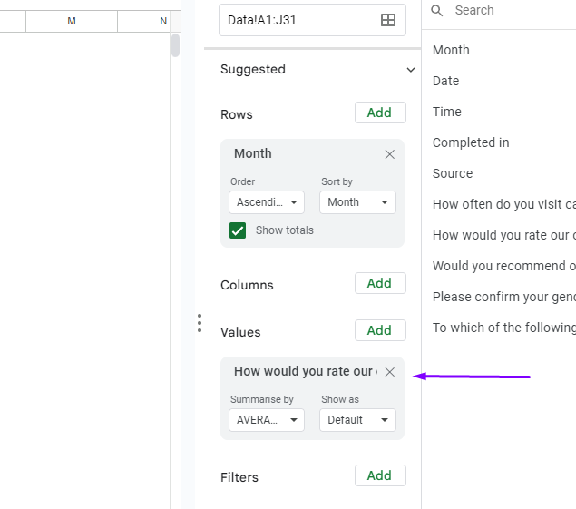
The most obvious thing to do would be to focus on numerical data which can be added or averaged in a straight-forward manner. The answers to ‘How would you rate our coffee?’ present us with such data since the respondents had to evaluate the café on a scale from 1-5.
In the Value section of the pivot table editor we choose this question.By default the pivot table shows the sum of values, but we are interested in the average for respectively January and February. First switch the calculation type to ‘average’.

Now you see that on average the clients gave the café 3.6 out of 5 the entire data set, i.e. January and February.
Let’s compare the data month over month. In rows choose ‘month’. You can also show the month in column but we go for row since it gives a better layout.

Now we can clearly see how customer satisfaction changes month over month.When working with a larger data set, you can follow how this metric fluctuates over time and if you spot big value changes that deviates from the average for the entire data set, you can try to associate them with specific events. For example, the fact that hiring an experienced new employee coincides with a surge in customer satisfaction suggests the new colleague has proven to be a good hire.
.
Example #2 - text strings
In the example above the answers were numerical. How to proceed if your data are text strings which cannot be selected as ‘value’ and simply added or averaged?
First, clean the ‘values’ section in the pivot table editor.
The month rows can stay as they are. Let’s use the question ‘Would you recommend our cafe to a friend or colleague?’ as an example. In the column section I select this question. The two answer alternatives appear in the column descriptions.
Now we need to populate the values. It may not be intuitive in the beginning, but we choose any metric from the table that has populated (filled in) cells. In our case there are no empty cells, but once you start working with more complex tables, it's important to keep that in mind. We choose ‘date’.
What the Pivot does it that it shows the number of times the date cell is populated for the rows that contain
- January and the answer is yes
- January and the answer is no
- February and the answer is yes
- February and the answer is no
Again, this sort of comparison makes most sense when
applied over a longer period of time so that you don’t get mislead by short time fluctuations
put in context with events influencing your business so that you can spot correlations

The example above shows you basic ways of comparing data using a Pivot table. We encourage you to explore this feature in your spreadsheet software. It’s a powerful tool that can be used for creating complex and yet clear presentations of large data sets and multiple metrics.